SQL Tuning: Thinking in Sets / How and When to be Bushy
November 5, 2015 5 Comments
Below is a SQL statement from a performance problem I was looking at the other day.
This is a real-world bit of SQL which has slightly simplified and sanitised but, I hope, without losing the real-worldliness of it and the points driving this article.
You don’t really need to be familiar with the data or table structures (I wasn’t) as this is a commentary on SQL structure and why sometimes a rewrite is the best option.
SELECT bd.trade_id
,      bdp.portfolio_id
,      bd.deal_id
,      bd.book_id
,      pd.deal_status   prev_deal_status
FROM   deals            bd
,      portfolios       bdp
,      deals            pd
,      portfolios       pdp
-- today's data
WHERE  bd.business_date         = :t_date
AND    bd.src_bus_date          < :t_date
AND    bd.type                  = 'Trade'
AND    bdp.ref_portfolio_id     = bd.book_id
-- yesterday's data
AND    pd.business_date         = :y_date
AND    pd.type                  = 'Trade'
AND    pdp.ref_portfolio_id     = pd.book_id
-- some join columns
AND    bd.trade_id              = pd.trade_id
AND    bdp.portfolio_id         = pdp.portfolio_id;
There is no particular problem with how the SQL statement is written per se.
It is written in what seems to be a standard developer way.
Call it the “lay everything on the table” approach.
This is a common developer attitude:
“Let’s just write a flat SQL structure and let Oracle figure the best way out.”
Hmmm… Let’s look at why this can be a problem.
First, what is the essential requirement of the SQL?
Compare information (deal status) that we had yesterday for a subset of deals/trades
Something like that anyway…
So … What is the problem?
The Optimizer tends to rewrite and transform any SQL we give it anyway and tries to flatten it out.
The SQL above is already flat so isn’t that a good thing? Shouldn’t there be less work for the optimizer to do?
No, not necessarily. Flat SQL immediately restricts our permutations.
The problem comes with how Oracle can take this flat SQL and join the relevant row sources to efficiently get to the relevant data.
Driving Rowsource
Let’s assume that we should drive from today’s deal statuses (where we actually drive from will depend on what the optimizer estimates / costs).
SELECT ...
FROM   deals            bd
,      portfolio        bdp
...
-- today's data
WHERE  bd.business_date         = :t_date
AND    bd.src_bus_date          < :t_date
AND    bd.type                  = 'Trade'
AND    bdp.ref_portfolio_id     = bd.book_id
....
Where do we go from here?
We want to join from today’s deals to yesterdays deals.
But the data for the two sets of deals data is established via the two table join (DEALS & PORTFOLIOS).

We want to join on TRADE_ID which comes from the two DEALS tables and PORTFOLIO_ID which comes from the two PORTFOLIOS tables.
SELECT ...
FROM   ...
,      deals            pd
,      portfolios       pdp
WHERE  ...
-- yesterday's data
AND    pd.business_date         = :y_date
AND    pd.type                  = 'Trade'
AND    pdp.ref_portfolio_id     = pd.book_id
...
And joined to via:
AND    bd.trade_id              = pd.trade_id
AND    bdp.portfolio_id         = pdp.portfolio_id
So from our starting point of today’s business deals, we can either go to PD or to PDP, but not to both at the same time.
Hang on? What do you mean not to both at the same time?
For any multi-table join involving more than two tables, the Optimizer evaluates the different join tree permutations.
Left-Deep Tree
Oracle has a tendency to choose what is called a left-deep tree.
If you think about a join between two rowsources (left and right), a left-deep is one where the second child (the right input) is always a table.
NESTED LOOPS are always left-deep.
HASH JOINS can be left-deep or right-deep (normally left-deep as already mentioned)
Zigzags are also possible, a mixture of left-deep and right-deep.
Below is an image of a left-based tree based on the four table join above.

Here is an execution plan which that left-deep tree might represent:
---------------------------------------------------------------
| Id  | Operation                               | Name        |
---------------------------------------------------------------
|   0 | SELECT STATEMENT                      |               |
|   1 |  NESTED LOOPS                         |               |
|   2 |   NESTED LOOPS                        |               |
|   3 |    NESTED LOOPS                       |               |
|   4 |     NESTED LOOPS                      |               |
|*  5 |      TABLE ACCESS BY ROWID            | DEALS         |
|*  6 |       INDEX RANGE SCAN                | DEALS_IDX01   |
|   7 |      TABLE ACCESS BY INDEX ROWID      | PORTFOLIOS    |
|*  8 |       INDEX UNIQUE SCAN               | PK_PORTFOLIOS |
|*  9 |     TABLE ACCESS BY INDEX ROWID       | DEALS         |
|* 10 |      INDEX RANGE SCAN                 | DEALS_IDX01   |
|* 11 |    INDEX UNIQUE SCAN                  | PK_PORTFOLIOS |
|* 12 |   TABLE ACCESS BY INDEX ROWID         | PORTFOLIOS    |
---------------------------------------------------------------

Predicate Information (identified by operation id):
---------------------------------------------------

   5 - filter("BD"."TYPE"='Trade' AND "BD"."SRC_BUS_DATE"<:t_date)
   6 - access("BD"."BUSINESS_DATE"=:t_date)
   8 - access("BD"."BOOK_ID"="BDP"."REF_PORTFOLIO_ID")
   9 - filter(("BD"."TYPE"='Trade' AND "BD"."TRADE_ID"="PD"."TRADE_ID"))
  10 - access("PD"."BUSINESS_DATE"=:y_date)
  11 - access("PD"."BOOK_ID"="PDP"."REF_PORTFOLIO_ID")
  12 - filter("BDP"."PORTFOLIO_ID"="PDP"."PORTFOLIO_ID")
Right-Deep Tree
A right-deep tree is one where the first child, the left input, is a table.
Illustration not specific to the SQL above:

Bushy Tree
For this particular SQL, this is more what we are looking for:
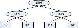
The essence of the problem is that we cannot get what is called bushy join, not with the original flat SQL.
The Optimizer cannot do this by default. And this isn’t an approach that we can get at by hinting (nor would we want to if we could, of course!).
Rewrite Required
To get this bushy plan, we need to rewrite our SQL to be more explicit around the set-based approach required.
WITH subq_curr_deal AS
     (SELECT /*+ no_merge */
             bd.trade_id
      ,      bd.deal_id
      ,      bd.book_id
      ,      bdp.portfolio_id
      FROM   deals      bd
      ,      portfolios bdp
      WHERE  bd.business_date         = :t_date
      AND    bd.src_bus_date          < :t_date
      AND    bd.type                  = 'Trade'
      AND    bdp.ref_portfolio_id     = bd.book_id)
,    subq_prev_deal AS
     (SELECT /*+ no_merge */
             pd.trade_id
      ,      pd.deal_status
      ,      pdp.portfolio_id
      FROM   deals      pd
      ,      portfolios pdp
      WHERE  pd.business_date         = :y_date
      AND    pd.type                  = 'Trade'
      AND    pdp.ref_portfolio_id     = pd.book_id)
SELECT cd.trade_id
,      cd.portfolio_id
,      cd.deal_id
,      cd.book_id
,      pd.deal_status prev_deal_status
FROM   subq_curr_deal cd
,      subq_prev_deal pd
WHERE  cd.trade_id             = pd.trade_id
AND    cd.portfolio_id         = pd.portfolio_id;
How exactly does the rewrite help?
By writing the SQL deliberately with this structure, by using WITH to create subqueries in conjunction with no_merge, we are deliberately forcing the bushy join.
This is an example execution plan that this bushy tree might represent.
----------------------------------------------------------
| Id  | Operation                        | Name          |
----------------------------------------------------------
|   0 | SELECT STATEMENT                 |               |
|*  1 |  HASH JOIN                       |               |
|   2 |   VIEW                           |               |
|   3 |    NESTED LOOPS                  |               |
|   4 |     NESTED LOOPS                 |               |
|*  5 |      TABLE ACCESS BY INDEX ROWID | DEALS         |
|*  6 |       INDEX RANGE SCAN           | DEALS_IDX01   |
|*  7 |      INDEX UNIQUE SCAN           | PK_PORTFOLIOS |
|   8 |     TABLE ACCESS BY INDEX ROWID  | PORTFOLIOS    |
|   9 |   VIEW                           |               |
|  10 |    NESTED LOOPS                  |               |
|  11 |     NESTED LOOPS                 |               |
|* 12 |      TABLE ACCESS BY INDEX ROWID | DEALS         |
|* 13 |       INDEX RANGE SCAN           | DEALS_IDX01   |
|* 14 |      INDEX UNIQUE SCAN           | PK_PORTFOLIOS |
|  15 |     TABLE ACCESS BY INDEX ROWID  | PORTFOLIOS    |
----------------------------------------------------------

Predicate Information (identified by operation id):
---------------------------------------------------

   1 - access("CD"."TRADE_ID"="PD"."TRADE_ID" AND "CD"."PORTFOLIO_ID"="PD"."PORTFOLIO_ID")
   5 - filter(("BD"."TYPE"='Trade' AND "BD"."SRC_BUS_DATE"<:t_date))
   6 - access("BD"."BUSINESS_DATE"=:t_date )
   7 - access("BD"."BOOK_ID"="BDP"."REF_PORTFOLIO_ID")
  12 - filter("PD"."TYPE"='Trade')
  13 - access("PD"."BUSINESS_DATE"=:y_date)
  14 - access("PDP"."REF_PORTFOLIO_ID"="PD"."BOOK_ID")
Is this a recommendation to go use WITH everywhere?
No.
What about the no_merge hint?
No.
The no_merge hint is a tricky one. This is not necessarily a recommendation but its usage here prevents the Optimizer from flattening. I often find it goes hand-in-hand with this sort of deliberately structured SQL for that reason, and similar goes for push_pred.
Do developers need to know about left deep, right deep and bushy?
No, not at all.
Takeaways?
It helps to think in sets and about what sets of data you are joining and recognise when SQL should be deliberately structured.
Further Reading
http://www.oaktable.net/content/right-deep-left-deep-and-bushy-joins
https://tonyhasler.wordpress.com/2008/12/27/bushy-joins/
https://www.toadworld.com/platforms/oracle/b/weblog/archive/2014/06/16/hitchhikers-guide-to-explain-plan-8
https://jonathanlewis.wordpress.com/2007/01/24/left-deep-trees/
https://antognini.ch/top/


Or you could just hang in there for a little bit longer and then upgrade: https://twitter.com/JLOracle/status/658804562313154560 😉
Thanks… started to read that yesterday and some patents from same author.
Or, in this particular case, you could just join once and then use an analytic function on the result:
select * from ( select d.trade_id, p.portfolio_id, d.deal_id, d.book_id, lead(d.deal_status) over( partition by d.trade_id, p.portfolio_id, d.deal_id, d.book_id order by d.business_date desc ) prev_deal_status from deals d, portfolios p where d.type = 'Trade' and d.book_id = p.ref_portfolio_id and d.src_bus_date < trunc(sysdate) and d.business_date in (trunc(sysdate), trunc(sysdate)-1) ) where prev_deal_status is not null;True.
The problem of oversimplification of the real world test case – unfortunately not true of the original. Well it is possible but perhaps not desirable due to the other different parameter for yesterdays data and today’s data.
🙂
Thanks.
Pingback: SQL Tuning : Thinking in Sets | Database Scene